Figures

Visual elements like images can significantly enhance the understanding of complex information at a glance. They add color and dynamics, offering a visual break from continuous, monotonous text, thus maintaining reader engagement. Therefore, do incorporate them effectively in your document to enrich the reader’s experience and aid in the comprehension of your material.

Criteria for Figures

Your figures should adhere to specific criteria:

• Content: Select content that is most relevant and illustrative of your point.
• Resolution: Opt for scalable vector graphics (such as SVG) or high-resolution images (minimum 300dpi). For diagrams or charts, consider using LaTeX-native graphics like TikZ or PGF.
• Colors: The choice of color depends on your printing method:
  • Colored: Use colors with significant contrast in hue, saturation, and lightness. You can find various color palettes online that suggest harmonious combinations. Ideally, choose palettes that are accessible to those with color vision deficiencies ^{1 2}. In your descriptions, opt for universally recognized color names like “dark red” or “light blue” rather than obscure ones.
  • Gray scale: If printing in gray scale, ensure adequate contrast between different shades. Avoid using very light grays as they might not print well. In diagrams, differentiate elements through distinct shapes or strokes, as you would with color.
• Dimensions: Figures do not necessarily have to span the entire page width. They should be appropriately scaled (e.g., to 60%) and centered.
• Scaling: Maintain consistent scale across similar types of figures, such as bar charts, ensuring uniform bar widths and font sizes.
• Labeling: Ensure that all diagrams are fully labeled, particularly the axes. Utilize legends or detailed captions to explain each component’s significance. Captions appear in the lists of figures and should be informative yet concise; if needed, provide a shortened version for lengthy descriptions.

Layout

LaTeX’s layout algorithms automatically place figures, tables, and listings in your text.

Unfortunately, these positions are not always ideal. Still, you should not waste time tweaking their positions throughout the writing process; it’s more efficient to adjust their placement only towards the end, once your full text is finished.

If you need to reposition these elements manually, it is advisable to position them preferably only at the top or only at the bottom of the page. This approach prevents isolated lines of text from getting sandwiched between them.

When multiple graphics are related or shall be compared, you can place them together on a special page. This page will then contain only graphics, no text.

In the figure, table and listings environments, prefer the position arguments t for top of the page, or p for a special page.

Simple figures

If you have an existing image, including it in your document is straightforward, as demonstrated with Figure 1. Additionally, it’s essential to accompany each image with a descriptive caption that explains the image’s content, including relevant details like colors, shapes, and groups. This is also the appropriate place to cite the source of the image using the \cite command if it is not originally yours. For the List of Figures, you may provide a shortened version of the caption if necessary. Lastly, assigning a label to the figure is crucial, as it enables you to refer to the figure elsewhere in your text efficiently. This approach ensures that your figures are not only well-integrated but also informative and correctly referenced.

\begin{figure}[t]
  \centering
  \includegraphics[width=.3\textwidth]{imgs/latex}
  \caption[Example figure]{An included image file showing the writing \LaTeX{}. Source: \cite{sample:wiki:latexlogo}}
  \label{fig:sample-latex}
\end{figure}

Subfigures

If you provide related figures, use subfigures as shown in Figure 2. Assign individual captions and labels to each subfigure and an overall caption and label for the entire group.

\begin{figure}[t]
  \centering
  \subcaptionbox
    [Black text on white background]
    {Black text on white background. Source: [1]}
    [.48\textwidth]
    {\includegraphics{samples/imgs/latex}}
  \hfill
  \subcaptionbox
    [White text on black background]
    {White text on black background. Adopted from: [1]}
    [.48\textwidth]
    {\includegraphics{samples/imgs/latex_dark}}
  \caption[Figure with two subfigures]
          {An example figure that contains two related subfigures.}
  \label{fig:subfigures}
\end{figure}

TikZ and PGF

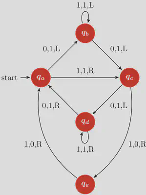
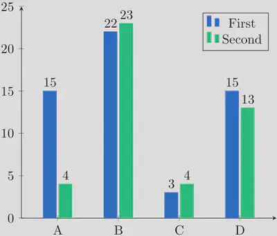
For creating graphs like those in Figures 3 and 4, consider using the TikZ and PGF packages. With these, similar to LaTeX, you simply supply the content and select a style; the layout is then generated automatically.

Many mathematics and statistics applications support direct export to TikZ and PGF formats. In R you can use the tikzDevice library and in Python projects with matplotlib you can use the tikzplotlib library to transform your graph into TikZ.

Note, TikZ consists of various libraries tailored for specific functionalities, so you may need to incorporate additional ones depending on your needs. To do this, include the necessary libraries using the command \usetikzlibrary in your main.tex file.

\begin{tikzpicture}[->,>=stealth',shorten >=1pt,auto,
    node distance=2.8cm,semithick]
  \tikzstyle{every state}=[fill=myred,draw=none,text=white,font=\boldmath]
  \node[initial,state] (A)                    {$q_a$};
  \node[state]         (B) [above right of=A] {$q_b$};
  \node[state]         (D) [below right of=A] {$q_d$};
  \node[state]         (C) [below right of=B] {$q_c$};
  \node[state]         (E) [below of=D]       {$q_e$};
  \path (A) edge              node {0,1,L} (B)
            edge              node {1,1,R} (C)
        (B) edge [loop above] node {1,1,L} (B)
            edge              node {0,1,L} (C)
        (C) edge              node {0,1,L} (D)
            edge [bend left]  node {1,0,R} (E)
        (D) edge [loop below] node {1,1,R} (D)
            edge              node {0,1,R} (A)
        (E) edge [bend left]  node {1,0,R} (A);
\end{tikzpicture}

\begin{tikzpicture}
  \begin{axis}[
      ybar,
      axis x line = bottom,
      axis y line = left,
      ytick pos = left,
      enlarge x limits  = 0.2,
      symbolic x coords = {A, B, C, D},
      nodes near coords,
      ymin = 0,
      ymax = 25,
      legend pos=north east
  ]
  \addplot[fill=myblue, draw=myblue] coordinates {
      (A, 15)
      (B, 22)
      (C, 3)
      (D, 15)
  };
  \addplot[fill=mygreen, draw=mygreen] coordinates {
      (A, 4)
      (B, 23)
      (C, 4)
      (D, 13)
  };
  \legend{First, Second}
  \end{axis}
\end{tikzpicture}